Decoding The Smith Chart: A Complete Information To Impedance Matching

Decoding the Smith Chart: A Complete Information to Impedance Matching

Associated Articles: Decoding the Smith Chart: A Complete Information to Impedance Matching

Introduction

On this auspicious event, we’re delighted to delve into the intriguing subject associated to Decoding the Smith Chart: A Complete Information to Impedance Matching. Let’s weave fascinating data and provide recent views to the readers.

Decoding the Smith Chart: A Complete Information to Impedance Matching

The Smith Chart, a seemingly advanced graphical device, is a cornerstone of radio frequency (RF) engineering. At first look, its intricate internet of circles and arcs might sound daunting, however beneath the floor lies a robust and stylish technique for visualizing and fixing impedance matching issues. This text will delve into the basics of the Smith Chart, explaining its development, interpretation, and sensible functions in RF circuit design.

Understanding the Fundamentals: Impedance and Reflection Coefficient

Earlier than embarking on the Smith Chart’s intricacies, we have to set up a agency grasp of two essential ideas: impedance and reflection coefficient.

• Impedance (Z): Impedance is the opposition to the move of alternating present (AC) in a circuit. It is a advanced amount, represented as Z = R + jX, the place:

  • R is the resistance (actual half), representing power dissipation.
  • X is the reactance (imaginary half), representing power storage in inductors (optimistic X) or capacitors (destructive X).

• Reflection Coefficient (Γ): When a transmission line is terminated with an impedance (Z_L) completely different from its attribute impedance (Z₀), a portion of the incident sign is mirrored again in direction of the supply. The reflection coefficient (Γ) quantifies this reflection:

  Γ = (Z_L – Z₀) / (Z_L + Z₀)

The reflection coefficient can be a fancy quantity, with a magnitude (|Γ|) representing the proportion of mirrored energy and an angle (∠Γ) indicating the section shift of the mirrored wave. A superbly matched load (Z_L = Z₀) leads to Γ = 0, which means no reflection.

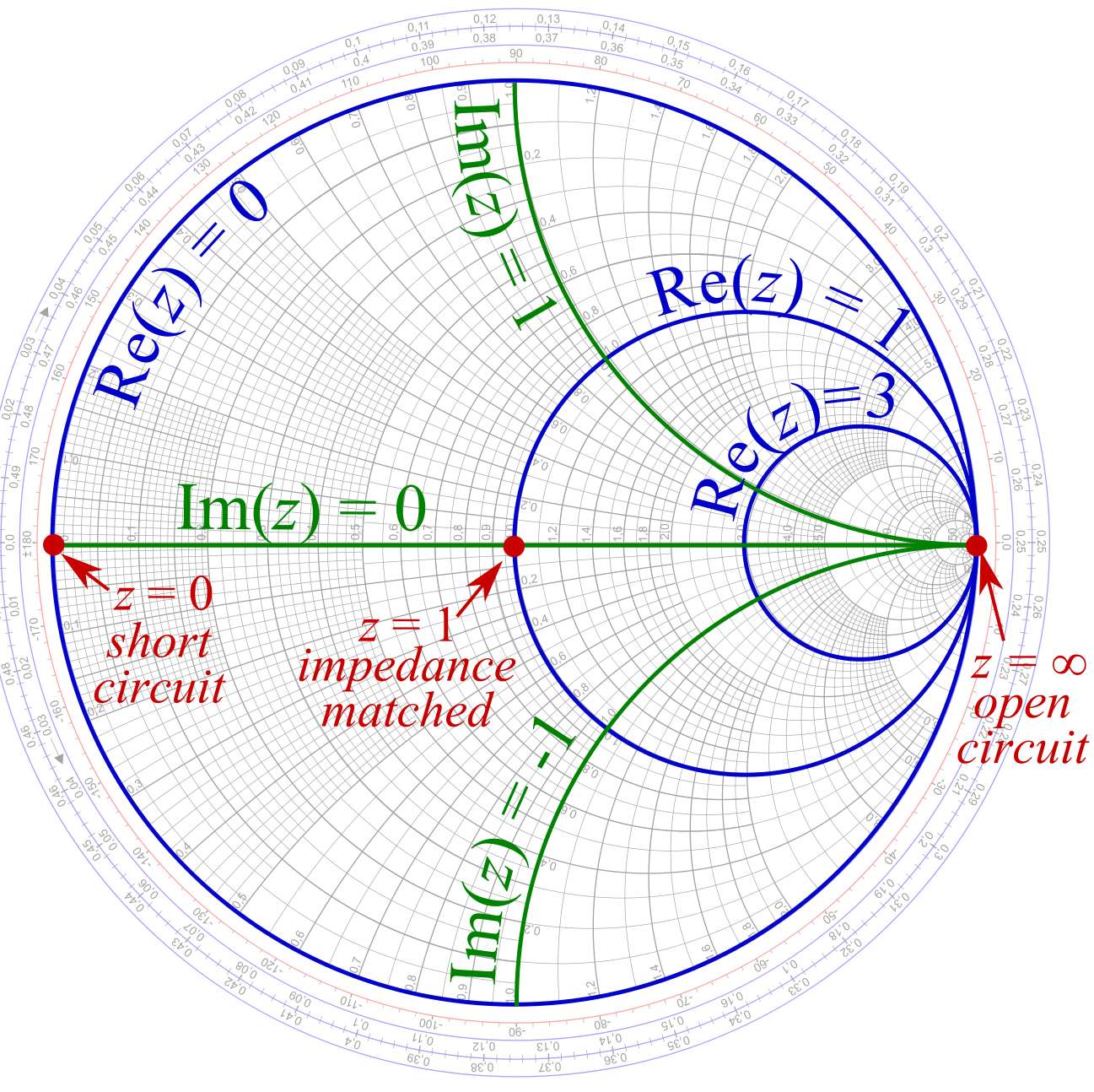
The Smith Chart’s Development: Mapping Impedance to Reflection Coefficient

The Smith Chart’s genius lies in its capacity to graphically signify the connection between impedance (or admittance) and the reflection coefficient. It is a polar plot the place:

• The middle represents an ideal match (Γ = 0). This corresponds to Z_L = Z₀.
• The circumference represents a complete reflection (|Γ| = 1). This happens when the load impedance is both open or short-circuited.
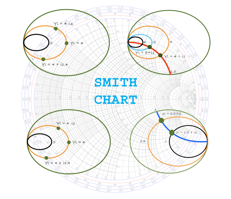
• Fixed resistance circles: These circles signify completely different values of resistance (normalized to Z₀). They’re centered on the horizontal axis (actual a part of Γ).
• Fixed reactance circles: These semi-circles signify completely different values of reactance (normalized to Z₀). They’re centered on the vertical axis (imaginary a part of Γ).

The Smith Chart is usually normalized to a attribute impedance of fifty ohms, a typical customary in RF methods. This normalization simplifies calculations by expressing impedances and admittances relative to Z₀. For instance, a 100-ohm impedance could be represented as 2 + j0 on a 50-ohm normalized Smith Chart.

Utilizing the Smith Chart for Impedance Matching:

The first utility of the Smith Chart is in impedance matching. The aim is to remodel the load impedance (Z_L) to match the attribute impedance (Z₀) of the transmission line, minimizing reflections and maximizing energy switch. That is sometimes achieved utilizing matching networks consisting of inductors and capacitors.

Here is how the Smith Chart facilitates this course of:

1. Find the Load Impedance: First, normalize the load impedance (Z_L) with respect to Z₀ and find it on the Smith Chart utilizing the fixed resistance and reactance circles.

2. Decide the Reflection Coefficient: The coordinates of the purpose representing Z_L immediately correspond to the magnitude and section of the reflection coefficient (Γ).

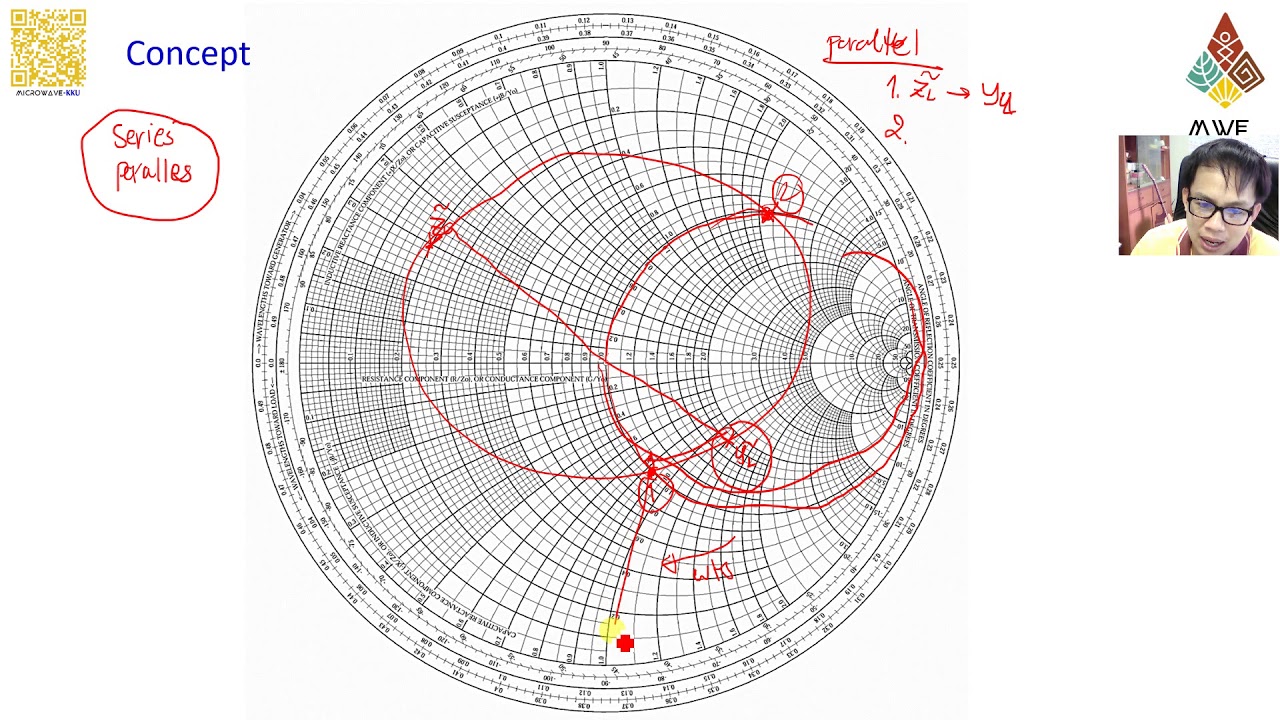
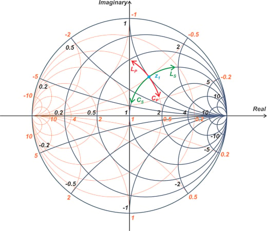
3. Matching Community Design: To attain a match, we have to transfer the impedance level in direction of the middle of the Smith Chart (Γ = 0). That is achieved by including reactive elements (inductors or capacitors) in collection or parallel with the load. Motion alongside fixed resistance circles represents including collection reactance, whereas motion alongside fixed conductance circles (obtained by inverting the impedance and plotting the admittance) represents including parallel reactance.

4. Iterative Course of: The method usually entails a number of steps, including elements and shifting the impedance level nearer to the middle with every iteration. The Smith Chart visually guides this iterative course of.

5. Transmission Line Size: The Smith Chart additionally incorporates the idea {of electrical} size, representing the bodily size of a transmission line part expressed in wavelengths. Shifting alongside a relentless impedance circle represents altering the size of a transmission line part. This can be utilized to successfully add or subtract reactance with out including discrete elements.

Past Impedance Matching: Different Functions

Whereas impedance matching is its main perform, the Smith Chart finds functions in numerous different RF engineering duties:

• Admittance Matching: By utilizing the admittance (Y = 1/Z) as an alternative of impedance, the Smith Chart can be utilized to design matching networks utilizing parallel elements.

• Analyzing Transmission Traces: The Smith Chart facilitates the evaluation of transmission line habits, together with standing wave ratios (SWR), reflection coefficients, and impedance transformations.

• Filter Design: The Smith Chart aids in designing and analyzing numerous forms of RF filters.

• Antenna Matching: Matching antennas to transmission traces is essential for environment friendly energy switch. The Smith Chart assists on this course of.

• Microwave Circuit Design: The Smith Chart is a useful device in designing and analyzing advanced microwave circuits.

Limitations and Alternate options:

Whereas extremely helpful, the Smith Chart has limitations:

• Graphical Nature: It depends on visible interpretation, which could be vulnerable to errors, particularly for advanced circuits.
• Normalized Values: Calculations should be normalized to Z₀, requiring cautious consideration to models.
• Restricted Accuracy: The accuracy will depend on the precision of the chart and the person’s capacity to learn it.

Trendy software program instruments provide refined circuit simulators and impedance matching calculators, usually changing the necessity for guide Smith Chart calculations. Nevertheless, understanding the Smith Chart stays invaluable for gaining an intuitive understanding of impedance matching and RF circuit habits. It gives a robust visible illustration that enhances numerical strategies.

Conclusion:

The Smith Chart, regardless of its seemingly intricate design, is a remarkably environment friendly and insightful device for RF engineers. Its capacity to graphically signify the connection between impedance, admittance, and reflection coefficient makes it indispensable for fixing impedance matching issues and gaining a deeper understanding of RF circuit habits. Whereas software program instruments have develop into more and more prevalent, mastering the Smith Chart stays an important talent for any RF engineer, providing a novel mix of visible instinct and sensible utility on the planet of high-frequency electronics. Understanding its rules permits for a extra intuitive grasp of the underlying physics, even when utilizing extra superior computational strategies. The visible illustration gives a robust examine and gives a framework for deciphering advanced simulations. Due to this fact, the Smith Chart continues to be a significant device within the RF engineer’s arsenal, providing a robust mix of visible instinct and sensible utility.

Closure

Thus, we hope this text has offered invaluable insights into Decoding the Smith Chart: A Complete Information to Impedance Matching. We hope you discover this text informative and helpful. See you in our subsequent article!