Mastering The Vary Bar Chart In Excel: A Complete Information

Mastering the Vary Bar Chart in Excel: A Complete Information

Associated Articles: Mastering the Vary Bar Chart in Excel: A Complete Information

Introduction

With nice pleasure, we are going to discover the intriguing subject associated to Mastering the Vary Bar Chart in Excel: A Complete Information. Let’s weave fascinating data and supply contemporary views to the readers.

Mastering the Vary Bar Chart in Excel: A Complete Information

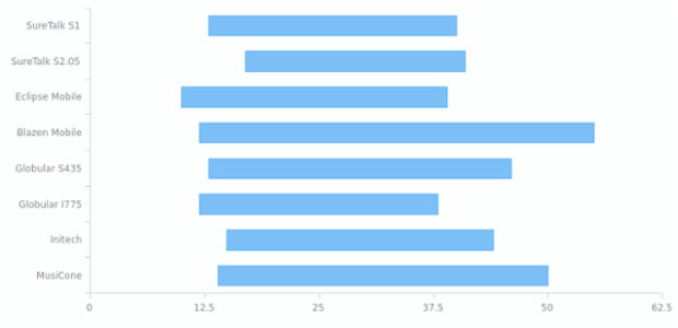
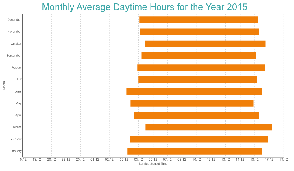
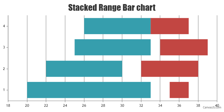
Vary bar charts, often known as high-low charts or vary charts, are highly effective visualization instruments that successfully show the vary or variation of knowledge inside specified classes. Not like easy bar charts that present a single worth per class, vary bar charts current each minimal and most values, offering a transparent image of the unfold and distribution. This makes them significantly helpful for showcasing information resembling inventory costs, temperature fluctuations, gross sales ranges, or any dataset the place the vary is a key facet of the data. This text gives a complete information to creating and customizing vary bar charts in Excel, overlaying varied strategies and superior options.

Understanding the Information Construction:

Earlier than diving into the creation course of, it is essential to know how your information needs to be structured for optimum outcomes. A spread bar chart wants at the least three columns of knowledge:

• Class: This column identifies the distinct teams or classes for which you are exhibiting the vary (e.g., months, product names, areas).
• Minimal Worth: This column incorporates the bottom worth for every class.
• Most Worth: This column incorporates the best worth for every class.

Elective columns can embrace:

• Common Worth: Including a median worth column can present additional context and insights into the central tendency of every class’s information.
• Different Metrics: You may embrace different related information factors, though visualizing them straight on the vary bar chart may turn out to be cluttered. Think about using information labels or a separate chart for extra metrics.

Methodology 1: Utilizing the Constructed-in Chart Function (Less complicated Information):

Excel gives a simple methodology to create vary bar charts in case your information is already structured as described above.

1. Put together Your Information: Arrange your information in a spreadsheet with the Class, Minimal Worth, and Most Worth columns. Guarantee your information is clear and freed from errors.

2. Choose the Information: Spotlight all three columns of knowledge, together with the headers.

3. Insert the Chart: Go to the "Insert" tab on the ribbon and navigate to the "Charts" part. Click on on the "Insert Column or Bar Chart" button and choose the "Clustered Column" chart sort. This may appear counterintuitive, however we’ll modify it shortly.

4. Convert to Vary Bar Chart: Proper-click on any of the bars within the chart and choose "Choose Information." Within the "Choose Information Supply" dialog field, click on on "Edit" underneath "Horizontal (Class) Axis Labels." Choose the "Class" column out of your information and click on "OK" twice. This step ensures your classes are appropriately displayed on the x-axis.

5. Modify Chart Collection: The chart presently shows two separate columns for minimal and most values. To mix them right into a single vary bar, right-click on one of many columns and choose "Change Collection Chart Kind." Select the "Excessive-Low" chart sort and click on "OK." This can remodel the clustered columns into a spread bar chart.

Methodology 2: Utilizing a Pivot Chart (Advanced Information):

For bigger datasets or information that requires aggregation or filtering, utilizing a PivotChart gives a extra versatile strategy.

1. Create a PivotTable: Choose your information vary and go to the "Insert" tab. Click on on "PivotTable" and select the place you wish to place the PivotTable (new worksheet or current one).

2. Configure the PivotTable: Drag the "Class" discipline to the "Rows" space. Drag the "Minimal Worth" discipline to the "Values" space. It’s best to see the minimal values displayed for every class.

3. Add Most Worth: Drag the "Most Worth" discipline to the "Values" space once more. Excel will routinely add it as a separate column.

4. Create the PivotChart: Click on wherever throughout the PivotTable. Go to the "Analyze" tab (or "PivotTable Analyze" in older variations of Excel) underneath the "PivotTable Instruments" part. Click on on "PivotChart" and select a chart sort. Choose the "Clustered Column" chart sort.

5. Convert to Vary Bar Chart (Similar as Methodology 1): Observe steps 4 and 5 from Methodology 1 to transform the clustered column chart to a spread bar chart.

Customizing Your Vary Bar Chart:

As soon as your vary bar chart is created, you’ll be able to customise it to boost its readability and visible enchantment.

• **Chart

Closure

Thus, we hope this text has offered helpful insights into Mastering the Vary Bar Chart in Excel: A Complete Information. We recognize your consideration to our article. See you in our subsequent article!